← Back to Blog

How a 1-hidden-layer ReLU network learns a continuous function

2026.5.9

The universal approximation theorem says that a network with a single hidden layer can approximate any continuous function arbitrarily well, given enough neurons. The classical proofs (Cybenko, Hornik) are abstract. Here is a concrete, geometric construction that explains how the network does it, in the simplest case: a $(1, n, 1)$ network with ReLU activation, learning a continuous function $f: [a, b] \to \mathbb{R}$.

Setup

Let the hidden-layer weights and biases be $w^{(1)}_j, b^{(1)}_j$ and the output-layer weights $w^{(2)}_j, b^{(2)}_j$, for $j = 1, \dots, n$. Each hidden neuron computes

$$h_j(x) = \mathrm{ReLU}\big(w^{(1)}_j x + b^{(1)}_j\big).$$

Define the kink point $q_j$ of neuron $j$ by $w^{(1)}_j q_j + b^{(1)}_j = 0$, i.e.

$$q_j = -\frac{b^{(1)}_j}{w^{(1)}_j}.$$

Without loss of generality take $w^{(1)}_j = 1,\ b^{(1)}_j = -q_j$ so $h_j(x) = \mathrm{ReLU}(x - q_j)$.

Two neurons make a ramp

Take two neurons $j, k$ with $q_j < q_k$. Then

$x < q_j$: $h_j(x) = h_k(x) = 0$
$q_j \le x \le q_k$: $h_j(x) = x - q_j,\ h_k(x) = 0$
$x > q_k$: $h_j(x) = x - q_j,\ h_k(x) = x - q_k$

Couple their output weights with opposite signs and equal biases:

$$w^{(2)}_k = -w^{(2)}_j =: w_{(j,k)}, \qquad b^{(2)}_j = b^{(2)}_k =: \tfrac{1}{2} b_{(j,k)}.$$

Their summed contribution to the output is

$$y_{(j,k)}(x) = w_{(j,k)} \big[h_j(x) - h_k(x)\big] + b_{(j,k)},$$

which evaluates to a "ramp":

$$y_{(j,k)}(x) = \begin{cases} b_{(j,k)}, & x < q_j \\ w_{(j,k)}(x - q_j) + b_{(j,k)}, & x \in [q_j, q_k] \\ w_{(j,k)}(q_k - q_j) + b_{(j,k)}, & x > q_k. \end{cases}$$

So a pair of ReLU neurons produces a function that is constant on $(-\infty, q_j)$, linear on $[q_j, q_k]$ with slope $w_{(j,k)}$, and constant again on $(q_k, \infty)$. Each such pair owns one linear segment.

Stitching pairs into a piecewise-linear approximation

Partition $[a, b]$ into $m = n/2$ equal sub-intervals of width $\delta = (b - a)/m$. For the $l$-th interval $[a + (l-1)\delta,\ a + l\delta]$, dedicate the pair $(2l-1, 2l)$ with

$$q_{2l-1} = a + (l-1)\delta, \quad q_{2l} = a + l\delta,$$ $$w_{(2l-1, 2l)} = \frac{f(a + l\delta) - f(a + (l-1)\delta)}{\delta}.$$

That is, set the slope of pair $l$ to the secant slope of $f$ on its interval. Each pair contributes the constant $w_{(2l-1, 2l)} \cdot \delta = f(a + l\delta) - f(a + (l-1)\delta)$ to the right of its interval. Telescoping over all pairs, for $x \in [a + (l-1)\delta,\ a + l\delta]$ the network output is

$$\sum_{l'=1}^{m} y_{(2l'-1,\, 2l')}(x) = f(a + (l-1)\delta) - f(a) + w_{(2l-1, 2l)}\big(x - a - (l-1)\delta\big) + \sum_{l'=1}^{m} b_{(2l'-1,\, 2l')}.$$

Choose the global offset $\sum_{l'} b_{(2l'-1,\, 2l')} = f(a)$ (e.g. put it all on the first pair) and the right-hand side becomes the linear interpolant of $f$ between its endpoint values on the $l$-th interval. As $\delta \to 0$ the piecewise-linear approximation converges uniformly to $f$. Continuous functions are well approximated by piecewise-linear ones, and ReLU networks are piecewise-linear by construction — that is the entire trick.

Does a trained network actually do this?

The construction above is a hand-built solution. A real network found by gradient descent need not parameterize itself this way. But the geometric claim is testable: after training, the network output should be piecewise-linear, with kinks exactly at $q_j = -b^{(1)}_j / w^{(1)}_j$, and the slope on $[q_l, q_{l+1}]$ should equal the secant slope of the target on that interval.

I trained a $(1, 200, 1)$ ReLU network with Adam for 20 000 steps to fit $f(x) = x^2$ on $[-1, 1]$, then read off all $q_j$ and the slope of each segment between consecutive kinks.

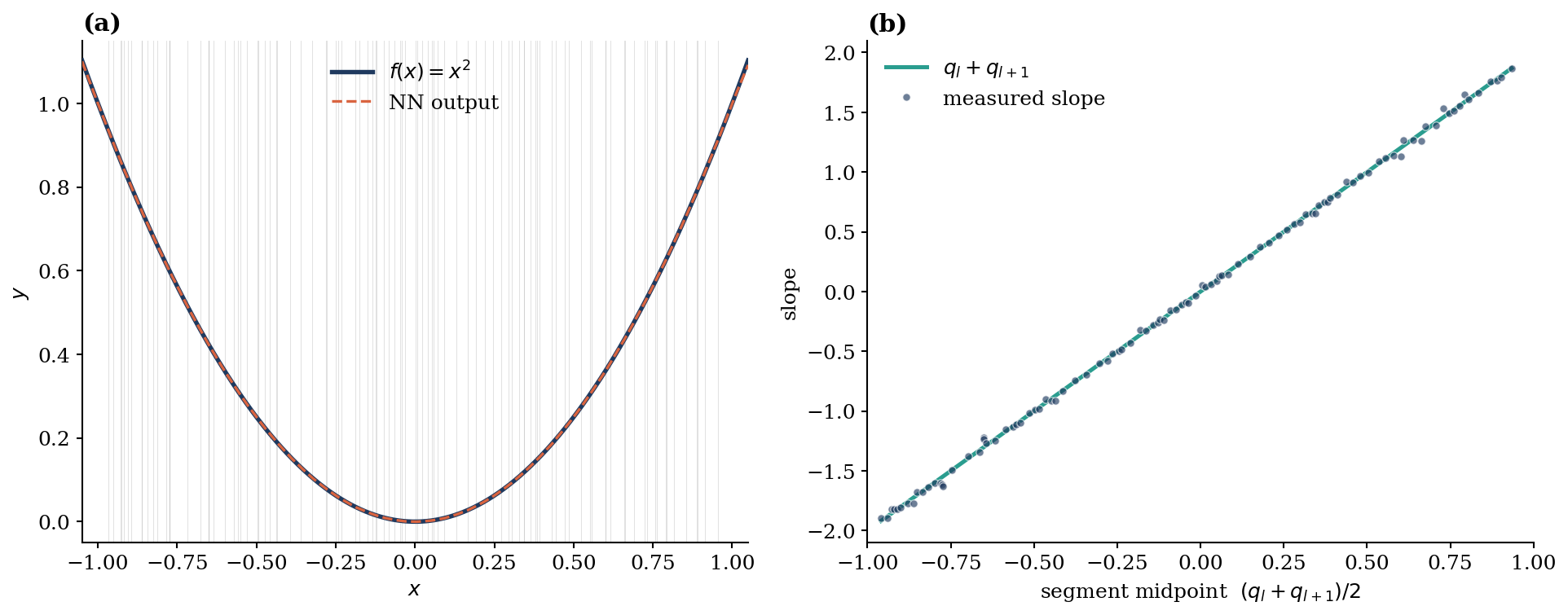
Trained NN matches x^2 with piecewise linear segments; segment slopes match q_l + q_{l+1}. — **(a)** The network output (orange dashed) is visually indistinguishable from $f(x) = x^2$ (navy). Gray vertical lines mark every kink $q_j = -b^{(1)}_j / w^{(1)}_j$; 101 of the 200 neurons place their kink inside $[-1, 1]$. **(b)** For each adjacent pair of in-domain kinks $(q_l, q_{l+1})$, the measured slope of the network on that segment (dots) is plotted against the segment midpoint. The teal line is the prediction from the construction: for $f(x) = x^2$, the secant slope on $[q_l, q_{l+1}]$ is $(q_{l+1}^2 - q_l^2)/(q_{l+1} - q_l) = q_l + q_{l+1}$. Median relative error: **1.6%**.

Two things to notice. First, the kinks distribute roughly uniformly on $[-1, 1]$ — which is exactly the optimal density for a function of constant curvature, since the optimal kink density for piecewise-linear approximation scales as $|f''|^{1/3}$, and $f''(x) = 2$ here. Second, the measured slopes lie on the line $y = 2 \cdot \text{midpoint}$ to within ~1.6% median error, confirming each segment is the chord of $x^2$ on $[q_l, q_{l+1}]$. The trained network has, in effect, discovered the construction above.

Half of the neurons place their kink outside $[-1, 1]$ and contribute only a linear function on the input domain. They do not waste capacity — they collectively account for the global offset and tilt of the approximation — but in a finite-data regime they are not where the model puts its representational power.

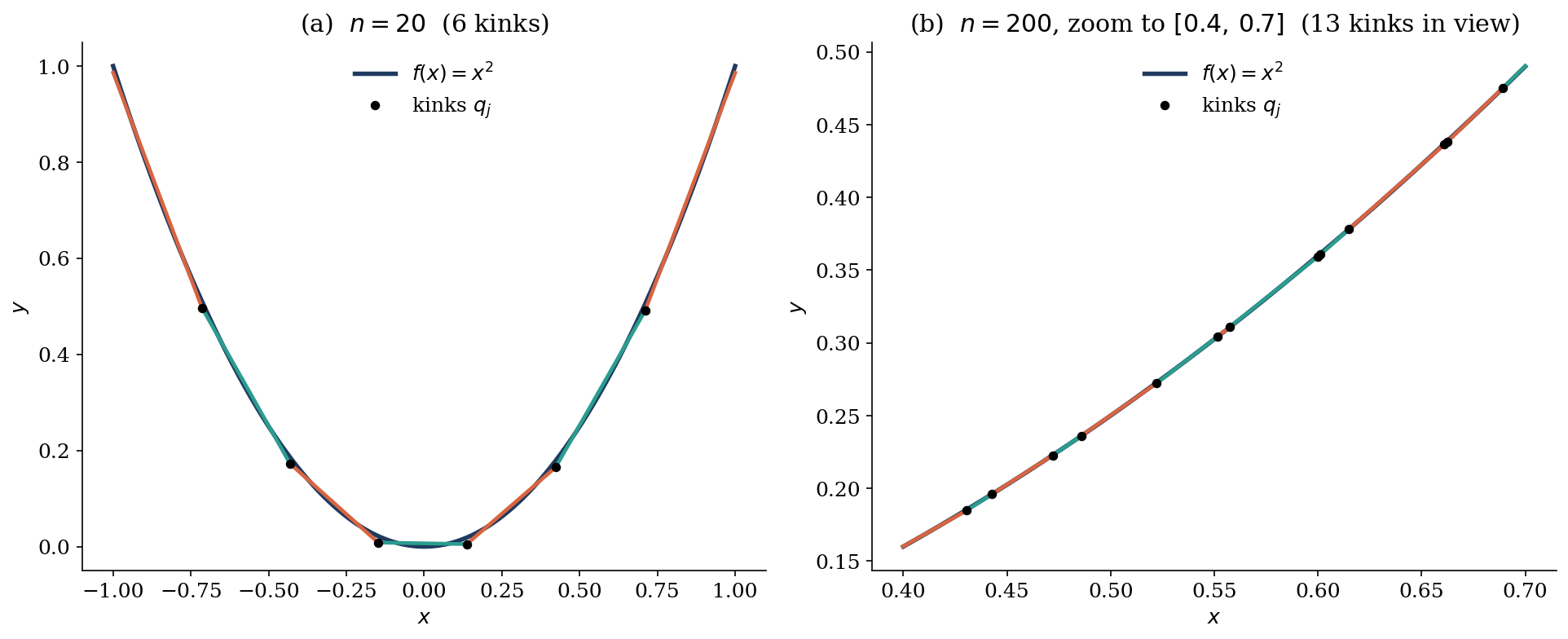
Seeing the strategy directly

The cleanest way to confirm the chord-by-chord picture is to plot, for each pair of adjacent kinks $(q_l, q_{l+1})$, the line that the network actually computes on that segment, and overlay $f(x) = x^2$. To make individual segments visible, I trained a smaller network ($n = 20$) and also include a zoom into a $(n = 200)$ network for comparison.

Each NN segment plotted as a chord of x^2; small n shows clear segments, large n zoom shows the same strategy at fine scale. — **(a)** A network with only $n = 20$ neurons places 6 kinks (black dots) inside $[-1, 1]$, partitioning the domain into 7 segments. On each segment the network is a single line — drawn in alternating orange/teal — which is exactly the chord of $x^2$ between the two adjacent kinks. Because $x^2$ is convex, every chord lies slightly above the parabola and meets it tangentially at the kinks. **(b)** Zooming a $n = 200$ network into $[0.4, 0.7]$ reveals the identical strategy at finer scale: the fit looks smooth from far away but is still a polygonal chain of chords up close. The strategy is invariant in $n$ — increasing $n$ just packs in more, smaller chords.

Why this is a useful picture

Stating universal approximation as "a smooth function is the limit of its piecewise-linear interpolants, and a ReLU network is exactly a piecewise-linear function" makes the result feel almost trivial — and it is, in 1D. The depth and difficulty in higher dimensions come from how kinks combine across multiple input axes, and from how compositional depth lets the number of linear regions grow exponentially with depth. But the 1D picture is the right starting intuition: the network is bending a continuous piecewise-linear surface to match data, one kink at a time.